Pipeline
Machine learning algorithms have become increasingly popular in recent years due to their ability to extract meaningful insights from large and complex datasets. Linear regression, clustering, and neural network are three popular machine learning algorithms that have been widely used in various fields such as finance, healthcare, and marketing.
Linear regression is a supervised learning algorithm that is used to predict a continuous outcome variable based on one or more predictor variables. Clustering is an unsupervised learning algorithm that is used to group similar objects together based on their characteristics. Neural networks are a type of machine learning algorithm that are inspired by the structure and function of the human brain and can be used for both supervised and unsupervised learning tasks.
In this section, we will provide an overview of these three machine learning algorithms, discuss their strengths and weaknesses, and provide examples of their applications. By understanding the strengths and weaknesses of different machine learning algorithms, practitioners can choose the most appropriate algorithm for their specific problem and data.
Data preparation
Preparing data is a crucial step in any machine learning project and can make a huge difference in terms of computational demand and accuracy of the model. Here, we cover the common types of features in machine learning models and 3 useful data preparation methods.
Types of features
-
Continuous variables: These variables represent numeric values that can take on any real value within a certain range. For example, variables like age, height, weight, temperature, or income are continuous variables.
-
Categorical variables: These variables represent discrete values that belong to a certain category or group. Categorical variables can be further classified into: Nominal variables (unordered categories without any inherent order or ranking, such as gender), Ordinal variables (with an inherent order or ranking among the categories, such as education level), Binary variables, Text or string variables, and Time-based variables. Text variables require special pre-processing techniques, such as text tokenization, feature extraction, and text encoding, before they can be used as inputs in machine learning models. Text variables are commonly used in natural language processing (NLP) tasks, such as sentiment analysis, text classification, or text generation.
Handling missing values
Missing values can occur in various forms, such as null values, NaN (Not a Number), or other placeholders in the dataset. Dealing with missing values properly is crucial as they can adversely affect the performance and accuracy of machine learning models if not addressed appropriately. Some common techniques for handling missing values in machine learning are:
Drop missing values: This is the simplest technique, but it can lead to loss of data. We can simply drop the rows or columns that contain missing values. However, this technique is only recommended when the missing values represent a small percentage of the data.
Imputation: Imputation involves filling in missing values with estimates such as mean, median, or mode of the non-missing values. Scikit-learn provides an Imputer class that can be used to impute missing values with different strategies.
Forward-fill or backward-fill: In some cases, it may be appropriate to use the value from the previous or next observation to fill in missing values. This technique is particularly useful when dealing with time series data.
Model-based imputation: Model-based imputation involves using a machine learning algorithm to predict missing values based on other variables in the dataset. This technique can be effective if there are strong correlations between the missing values and other variables in the dataset.
Create a new category: In categorical variables, we can create a new category to represent missing values. This technique can be useful if the missing values represent a significant portion of the data.
Feature scaling
Feature scaling is the process of transforming data to be on a similar scale or range. In machine learning, it is important to scale the features because many algorithms are sensitive to the scale of the input data.
There are two common techniques for feature scaling:
Standardization: In this technique, we transform the data so that it has zero mean and unit variance. The formula for standardization is:
Input
(x - mean(x)) / std(x)
Here, x is the feature, mean(x) is the mean of the feature, and std(x) is the standard deviation of the feature.
Min-max scaling: In this technique, we transform the data to have a range between 0 and 1. The formula for min-max scaling is:
Input
(x - min(x)) / (max(x) - min(x))
Here, x is the feature, min(x) is the minimum value of the feature, and max(x) is the maximum value of the feature.
It is important to note that the choice of scaling technique depends on the type of data and the machine learning algorithm being used. For example, if the algorithm assumes that the data is normally distributed, then standardization may be more appropriate. Conversely, if the algorithm requires the data to be between 0 and 1, then min-max scaling may be more appropriate.
Feature selection
Feature selection is the process of selecting a subset of the most relevant features (or variables) from a larger set of available features in a dataset, with the goal of improving the performance of a machine learning model.
In machine learning, having too many features can lead to overfitting, where the model is too complex and captures noise in the data, resulting in poor generalization to new data. Feature selection helps to reduce the dimensionality of the data, which can improve the performance of the model by reducing overfitting, decreasing the training time, and improving the interpretability of the model.
It is important to note that feature selection should be performed carefully, as removing important features can negatively impact the performance of the model. Therefore, it is important to evaluate the performance of the model with and without feature selection and choose the subset of features that results in the best performance.
Model evaluation
Once a model is trained, it needs to be evaluated to measure its performance. Model evaluation is a critical step in the machine learning workflow as it helps determine the quality of a trained model and its ability to make accurate predictions or decisions on new, unseen data. Some common techniques for model evaluation include cross-validation, where the model is trained and evaluated on multiple subsets of the data, and holdout evaluation, where a portion of the data is reserved for testing. Model evaluation also involves visualizing and analyzing the model’s predictions, error rates, and other performance metrics. The choice of metric depends on the type of problem, such as classification or regression, and the desired outcome of the model.
Overfitting occurs when a machine learning model learns to perform well on the training data but fails to generalize to new, unseen data. This means that the model may have learned the training data too well, including noise or irrelevant patterns, and fails to generalize to new data. Overfitting can result in a model that has high accuracy on the training data but performs poorly on test data or real-world data. Underfitting occurs when a machine learning model fails to capture the underlying patterns or complexity in the training data. Underfitting can occur when a model is too simple or lacks the capacity to learn the relevant patterns in the data.
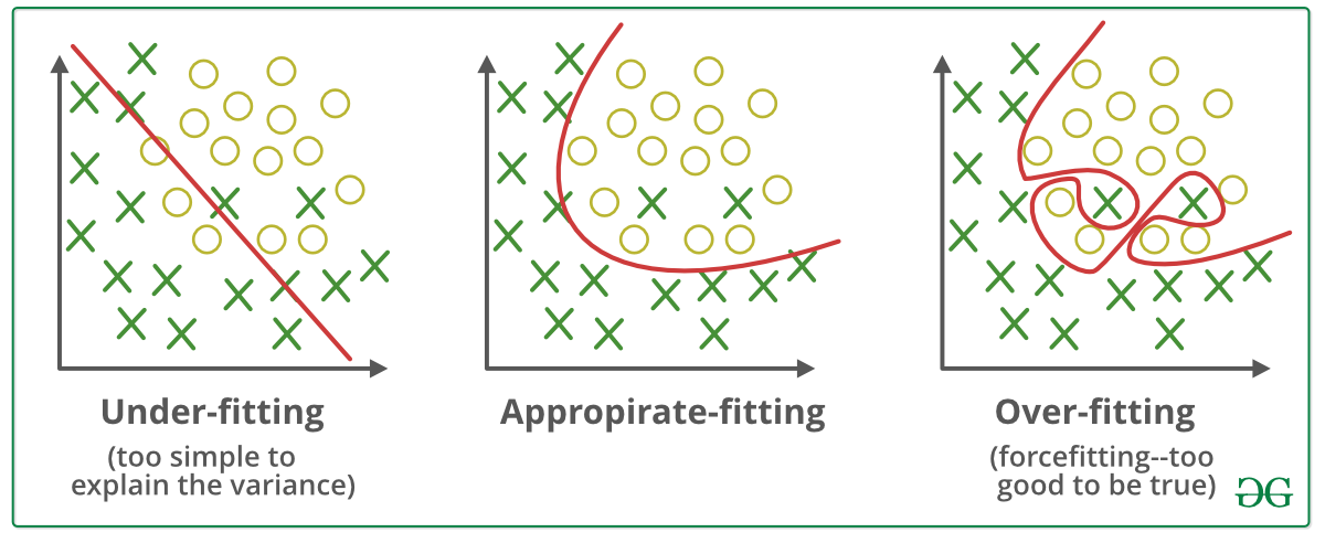
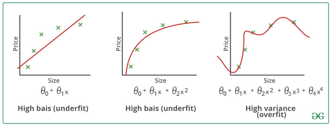 Image From: https://www.geeksforgeeks.org/underfitting-and-overfitting-in-machine-learning/
Loading last updated date...