Tasks
Table of contents
Introduction
Intro
Getting familiar with basic objects in Excel
Step 1
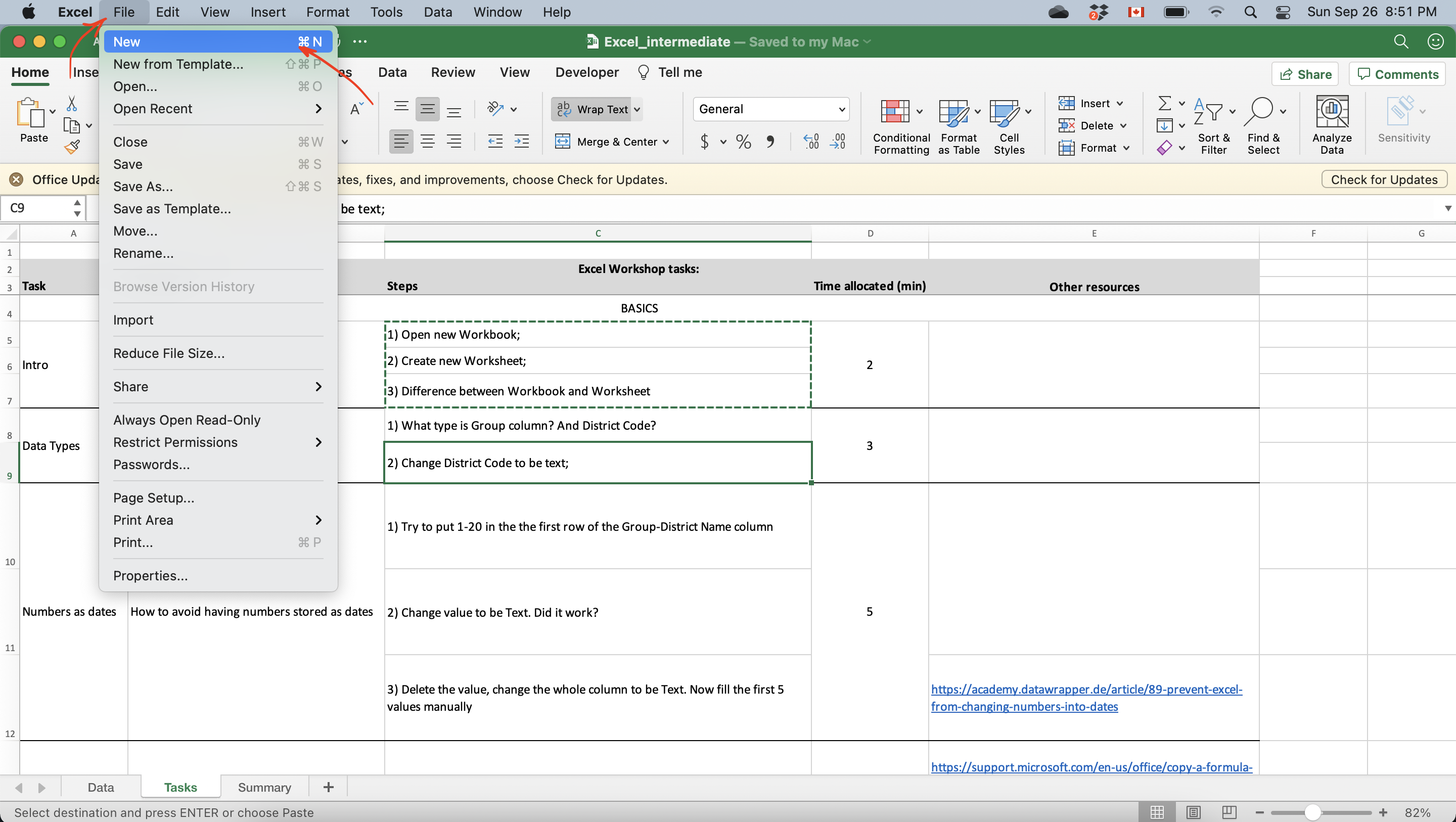
- Open new workbook.
- Choose File -> New in the Excel menu or press Ctrl+N (Cmd+N on Mac)
Step 2
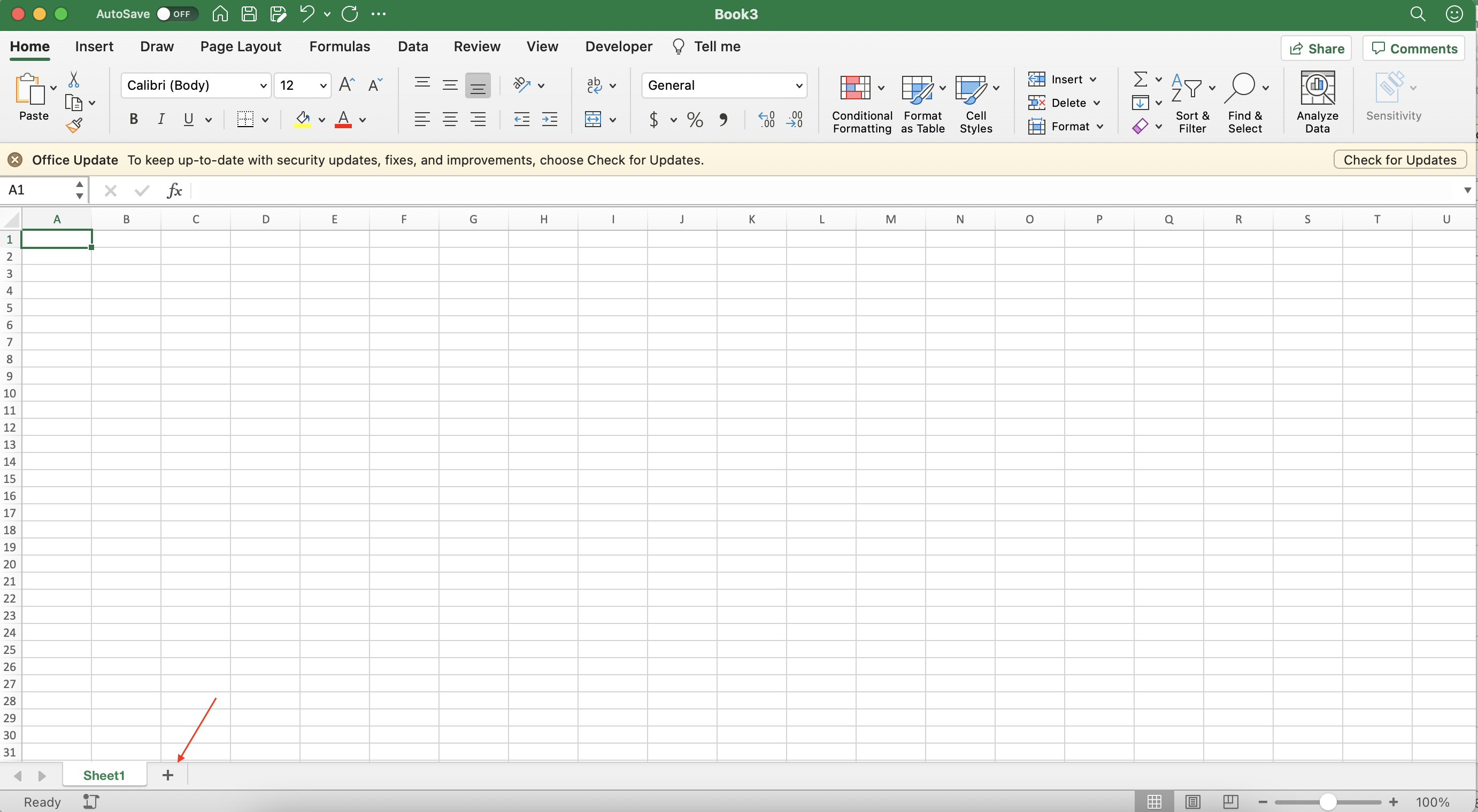
- Create new worksheet.
- In the opened workbook click on a plus in the bottom panel on the left
Step 3
Read more about difference between Workbook and Worksheet objects Geek Excel
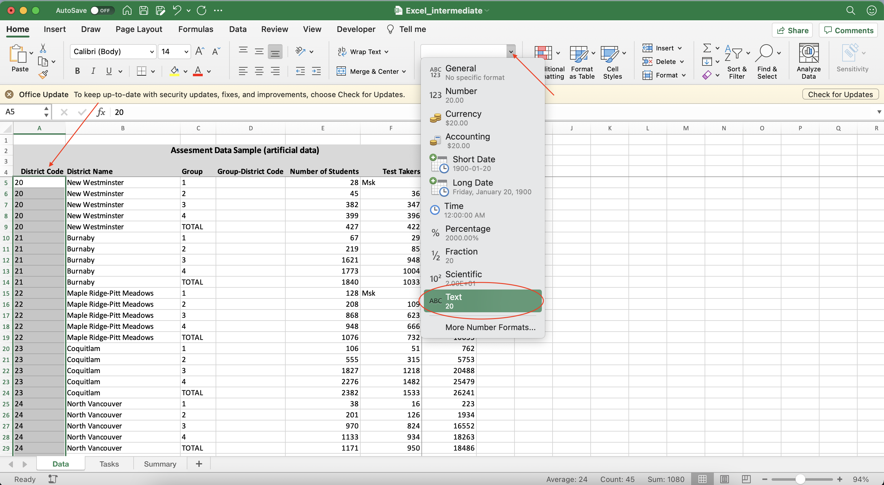
Data Types
Switching between data types
Most of the data is defined as a General type, unless specified otherwise. To learn what type a specific column is, select the range of values and check the dropdown list value in the Home tab.
Hint: the default alignment used by Excel suggests the data type too: numbers are aligned to the right, while text is aligned to the left.
Step 1
What type is Group column?
Step 2
What type is District Code column?
Step 3
Change District Code column to be Text.
Select values in District Code column (or select all the values in the column by clicking on the A in the column names pane) and then select Text instead of General
Number as Dates
How to avoid having numbers stored as dates
Step 1
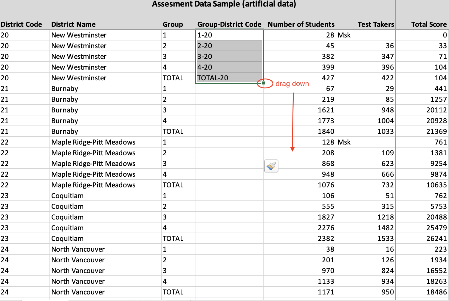
Try to put 1-20 in the first row of the Group-District Code column
Step 2
- Select filled cell (
D5) and change type to be Text. Did it work? - Unfortunately, Excel does not allow to switch between dates and text after the transformation has been done. However, we may prevent the automatic switch to the date format by choosing the format of column.
Step 3
Delete the value in the cell. Change the Group-District Code column to be Text. Now. fill the first 5 values manually following the pattern (1-20, 2-20,3-20, 4-20,TOTAL-20 ).
Link: Prevent Excel from changing numbers into dates
Autofill
How to fill values based on the pattern
We now can fill the rest of the patern using Autofill option.
Hint: you can also use CONCAT formula to fill the pattern using values from Group and District Name columns. Please note, that in this case you need to change column type to be General for the formula to work.
Step 1
Select first 5 rows of Group-District Code column and drag the fill handle down
Link: Microsoft guide on using autofill
Sorting
Explore existing sorting options
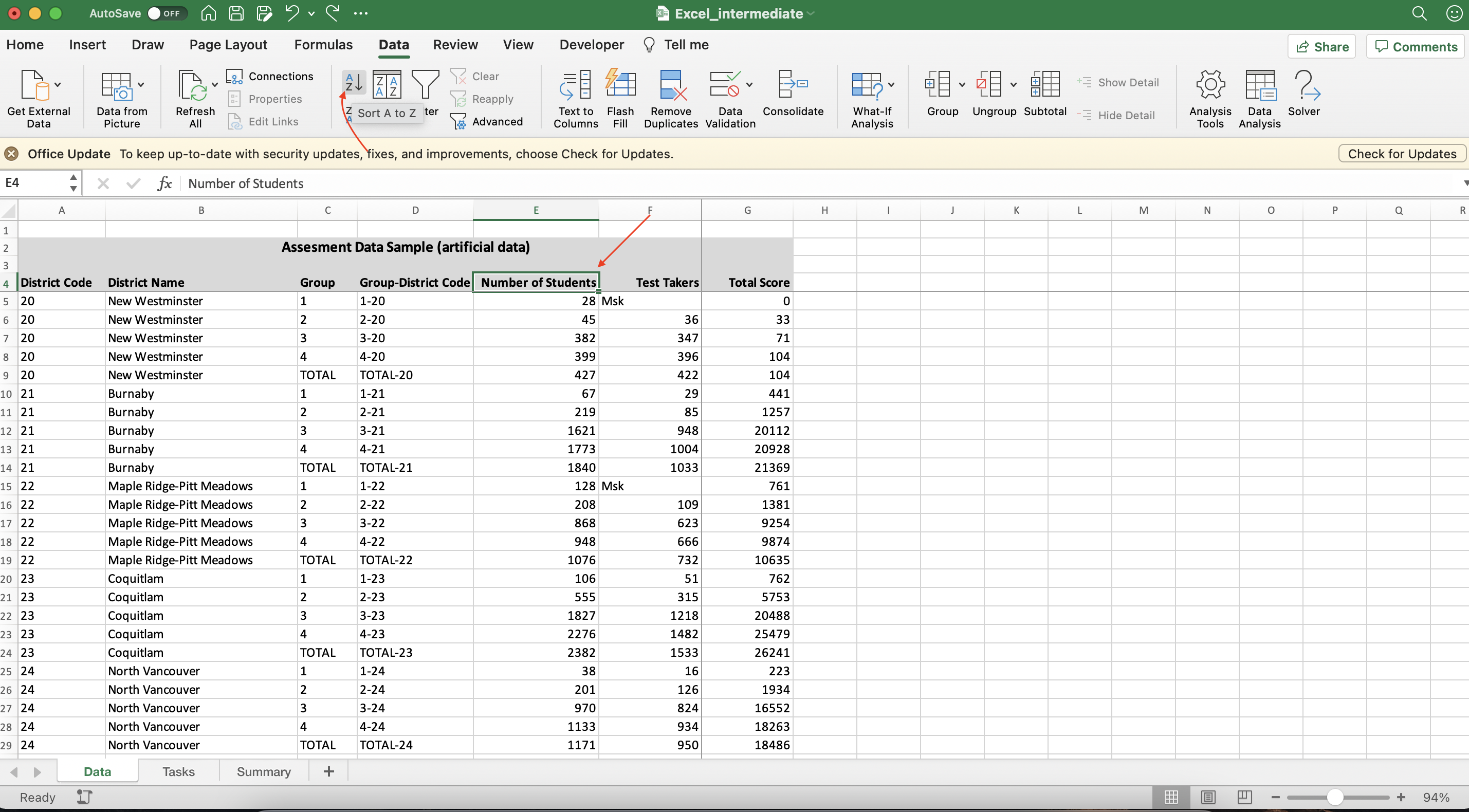
Step 1
- Sort data by the total number of students (ascending order).
- Select the
Number of Studentscolumn header (cellE4) and click Sort A to Z in the Data menu tab.
Hint: Applying Filter allows to use different sorting options as well
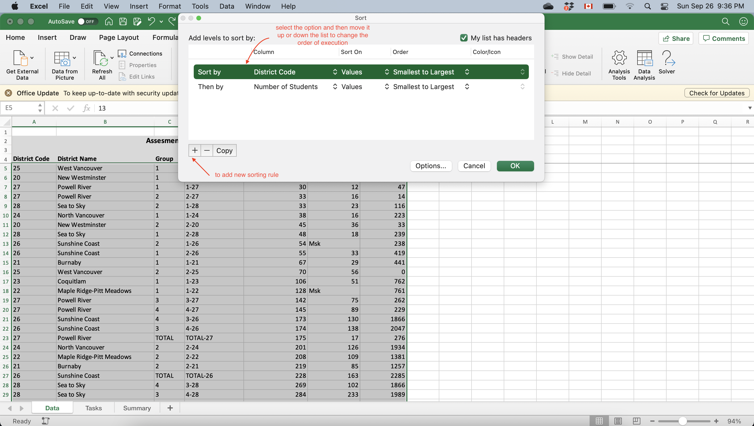
Step 2
- Add another level of sorting,
District Code. - Follow the previous step now for
District Codecolumn, or use Sort option in the Data menu to add several rules and change their hierarchies.
Filter
Removing errors using Filter
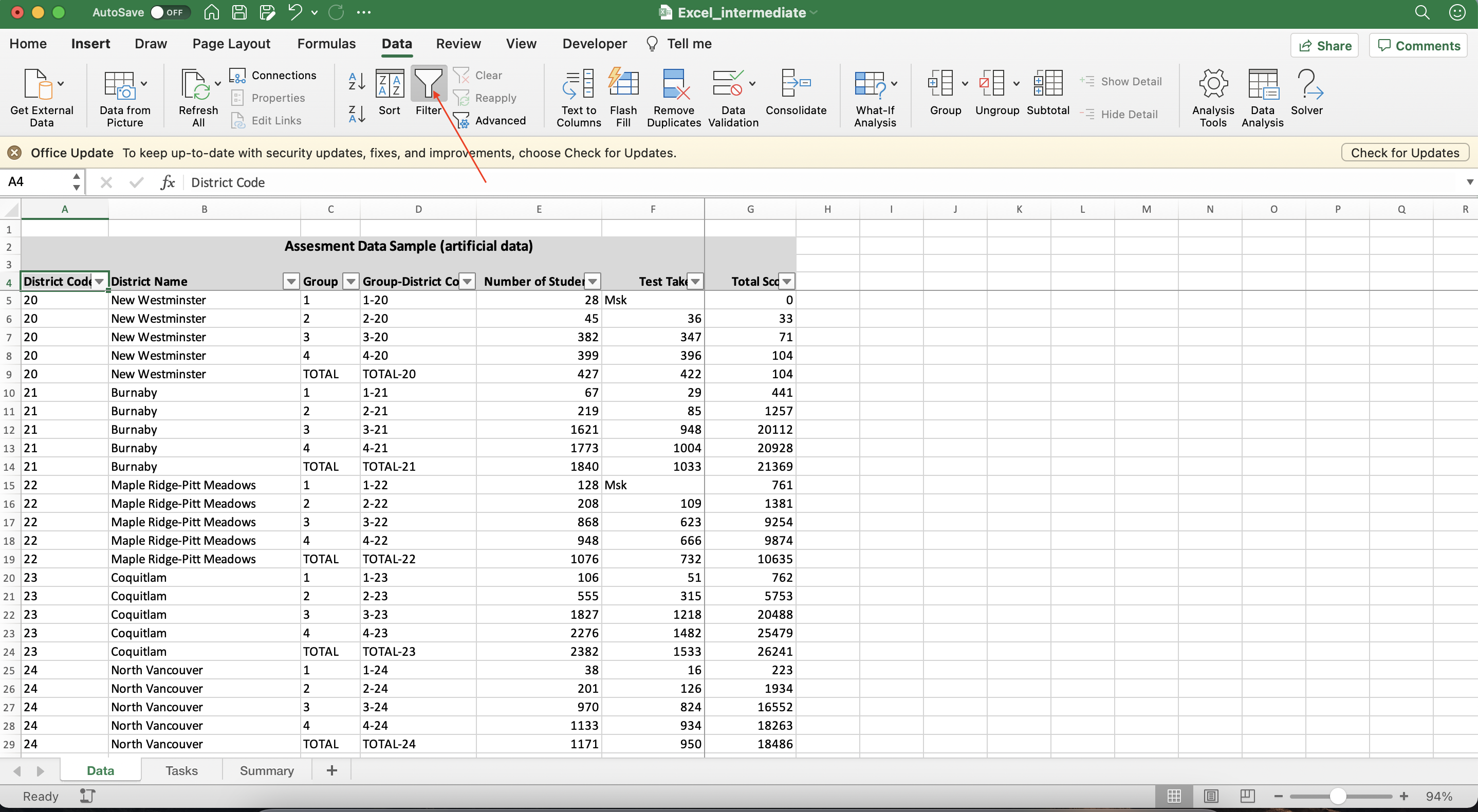
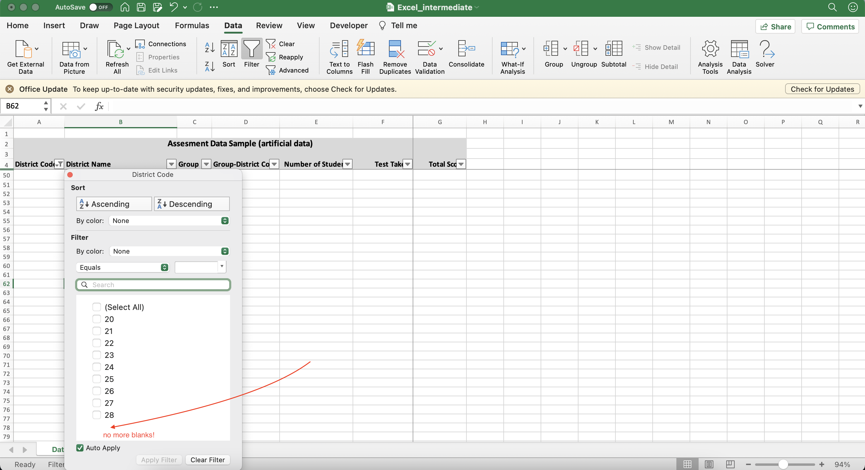
Step 1
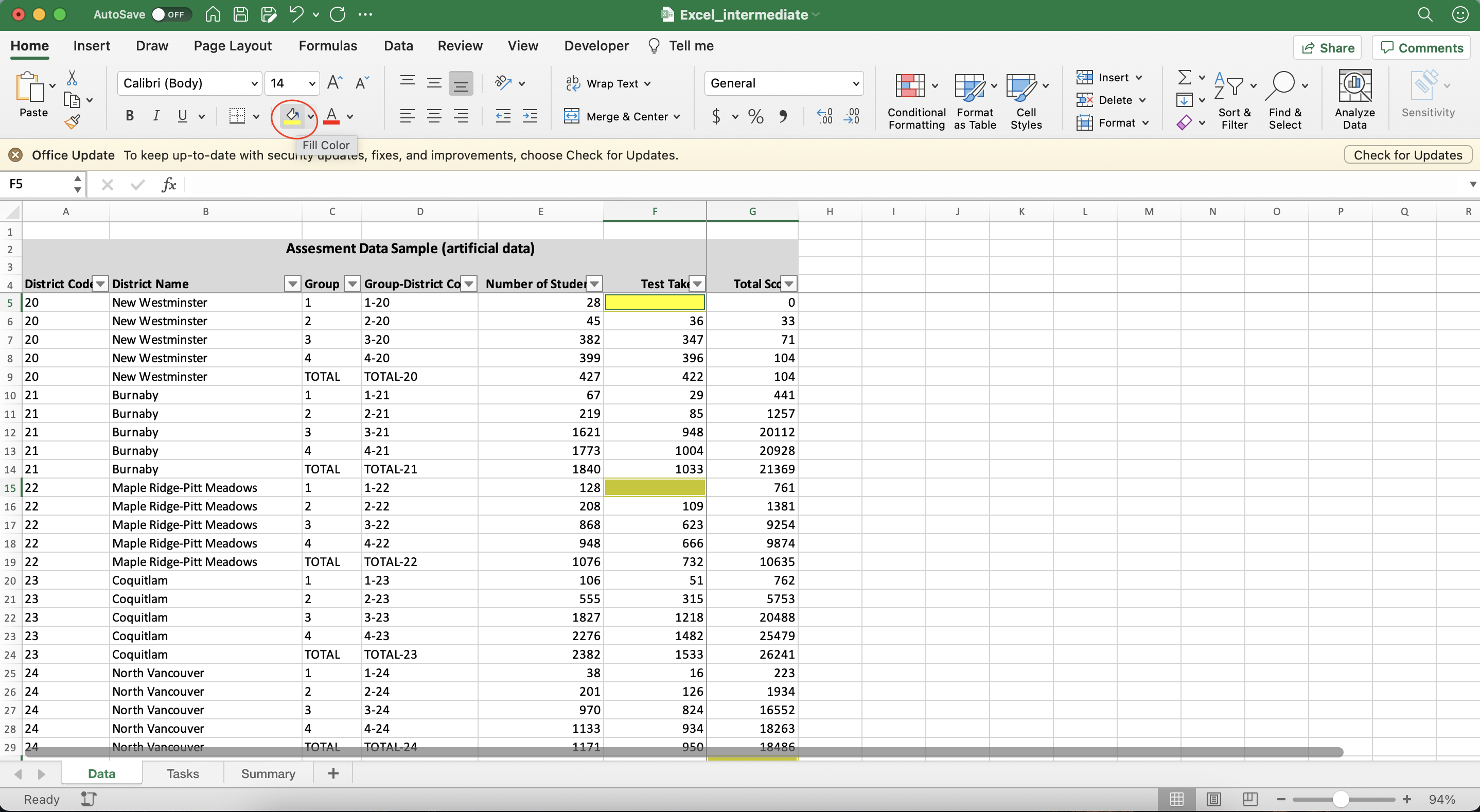
Apply Filter (located in the Data menu) to the District Code column.
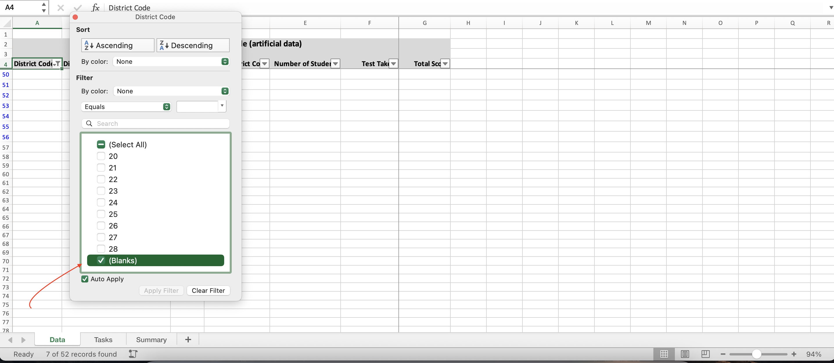
Step 2
Select rows with blank District Code
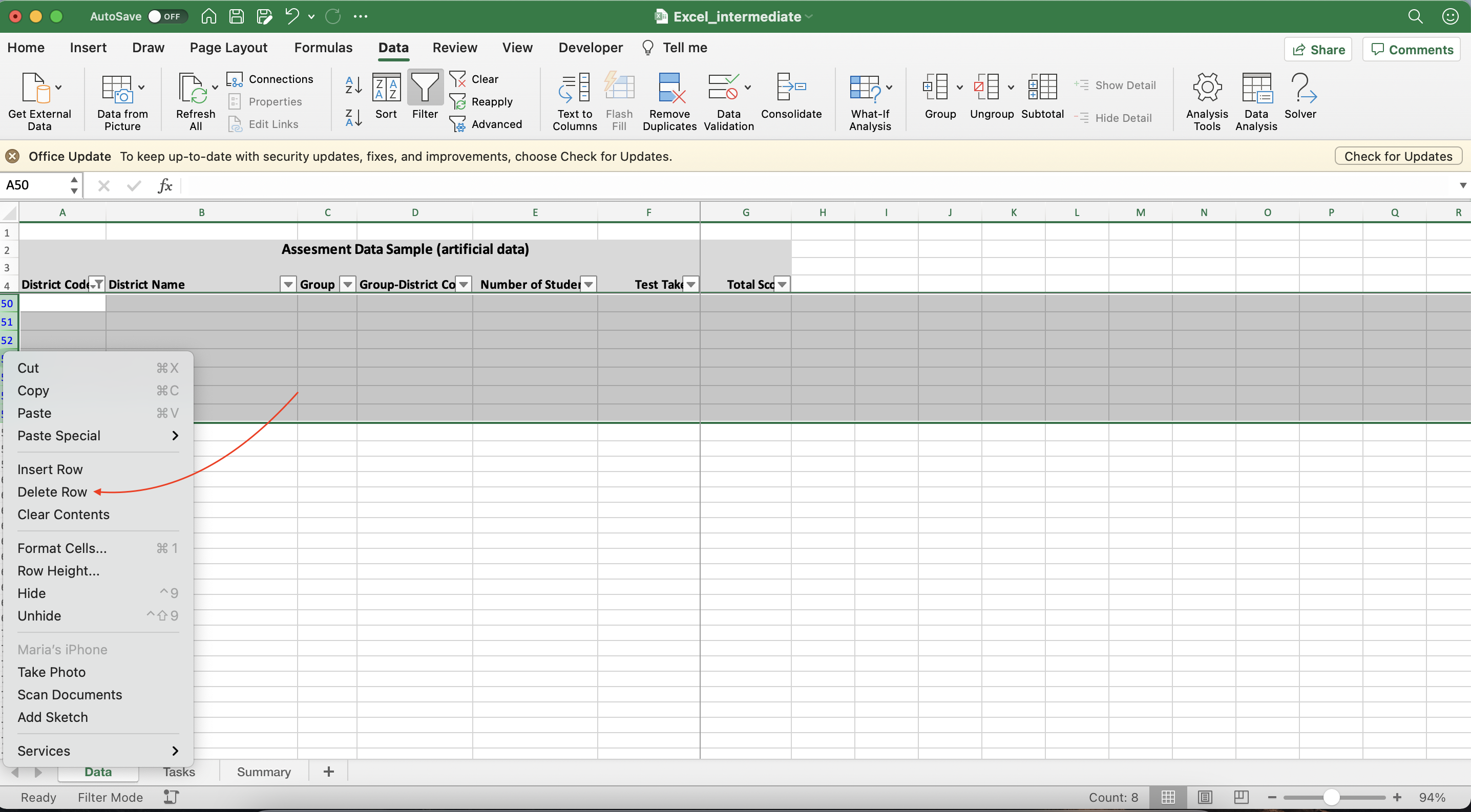
Step 3
Right click on selected rows and select option “Delete Rows”
Step 4
Make sure you do not have any blanks left
Link: 3 ways to remove empty rows
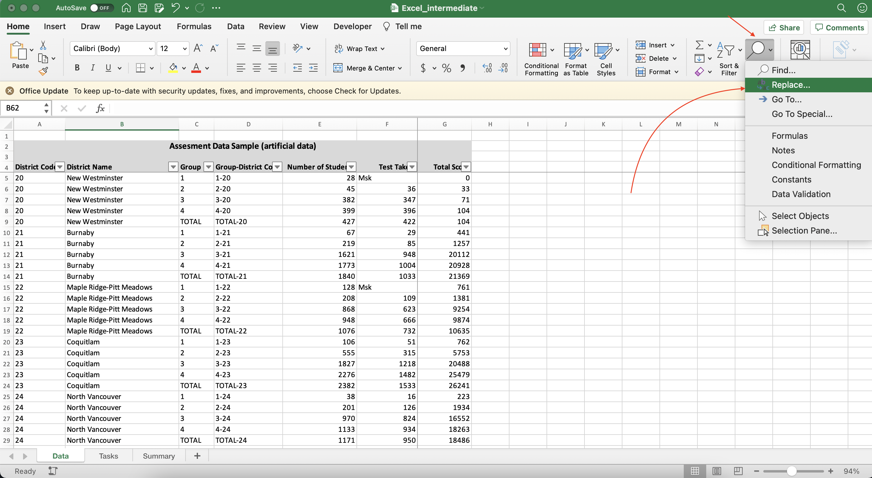
Find and Replace
Working with missing or masked values
Step 1
- Use Replace to find all “Msk” entries
- In the Find&Select option of main menu select Replace option or click Ctrl+H (both for PC and Mac);
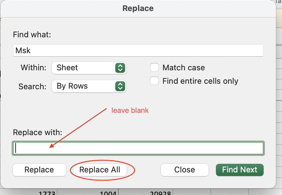
Step 2
- Replace “Msk” with blank.
- Do not put anything in the Replace field, not even a space
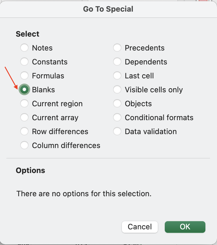
Step 3
- Use Go-To-Special to highlight blank cells
- Select the table area (not including headers) and select Go To Special from the Find&Select options. Click Fill Color to highlight selected cells
Link: Filling empty cells using Go To Special
Formulas
Intro to Formulas
Using SUM, AVG, COUNT
Hint: instead of using the formulas directly, you can also see these metrics (count, avg, sum) in the bottom right corner of the working area when selecting any range.
Step 1
Count how many observations contain number of test takers
Answer (click to open)
`COUNT(F5:F49)`
Step 2
Calculate total sum of the Number of Student column
Answer (click to open)
`SUM(E5:E49)`
Step 3
Find the average value of the Score column
Answer (click to open)
`AVG(G5:G49)`
Link: Basic Excel Formulas
Link: When to use absolute and relative references
Logical Functions
Calculate some metric if condition is true
Step 1
Create a new column Percent of Test Takers
Step 2
Use IF to get the percent of test takers for the Total values only:
Answer (click to open)
`IF(C5="TOTAL",F5/E5,"")`
Conditional Summary
Using SUMIF and SUBTOTAL
SUMIF is a conditional summary, which works identical to the SUM function when a certain condition is true. SUBTOTAL is used to calculate different aggregate functions (sum, avg, etc.). Use 1 as the first parameter to calculate average.
Step 1
Open Summary sheet
Step 2
Get the total number of test takers using SUMIF();
Hint: Use “Data!” in front of the cell name (e.g. Data!C2) to reference a cell from the sheet named Data.
Answer (click to open)
`SUMIF(Data!C5:C49,"TOTAL",Data!F5:F49)`
Step 3
Get the total number of test takers in Burnaby and Coquitlam using SUBTOTAL() .
Hint: Filter the table to select only rows related to these two districts.
Answer (click to open)
`SUBTOTAL(9,Data!F5:F49)`
VLOOKUP
Step 1
Return to the Summary sheet
Step 2
Use VLOOKUP to fill the rest of the summaries. Use absolute reference ($) to search rows from 5 to 49.
Hint: If VLOOKUP does not provide the right numbers, make sure to set the last parameter to be FALSE to get the exact match.
Answer (click to open)
`VLOOKUP(A9,Data!$D$5:$E$49,2,FALSE)`
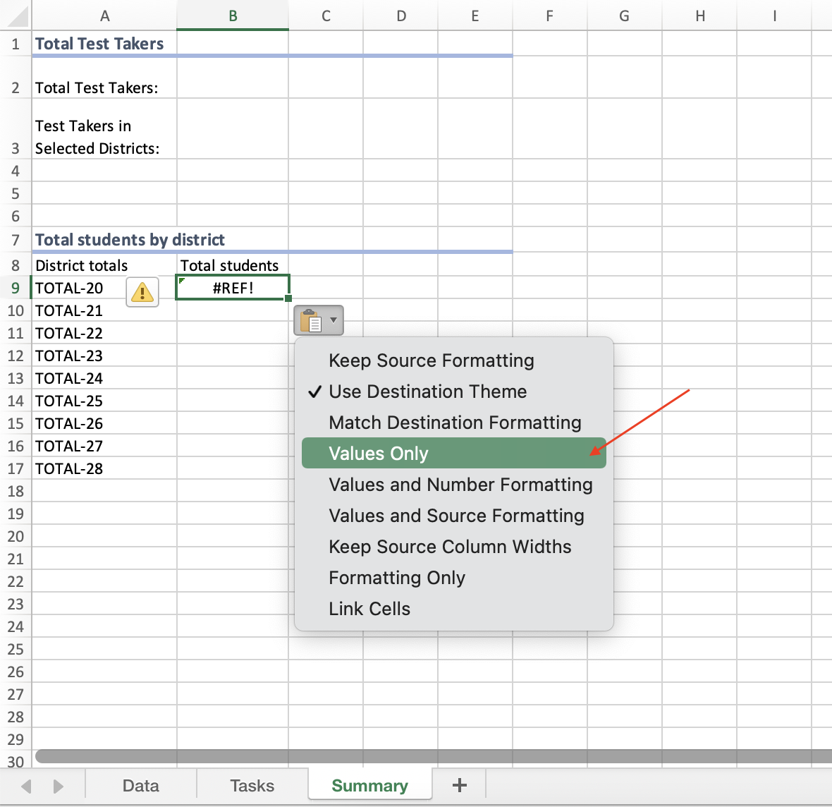
Smart Paste
Step 1
Copy the Percent of test takers values from the Data sheet into the Summary sheet.
To avoid messing up formula, use Smart Paste -> Values Only.
Hint: You can also subselect the TOTAL values only using Filter and then copy and paste a set of values as a range rigght into the Summary sheet.
Summaries and Visuals
Quick Analysis
Using Analyze Data Tool
NOTE: This option may not be avaliable in the older Excel versions or in the Office 365.
Step 1
Return to the Data sheet
Step 2
Select all your data and choose “Analyze Data” on the right
Step 3
Explore various options and choose what you think is appropriate!
Link: More on the Analyze Data tool and how to make most out of it
Pivot Table
Creating a simple Pivot Table
Step 1
Select Pivot Table from the Insert menu
Step 2
Select all columns in the table and choose to place the pivot table in the new worksheet
Step 3
In the opened worksheet, in the pane on the right select fields District Name, Test Takers and Total Score . Do you think this numbers are correct?
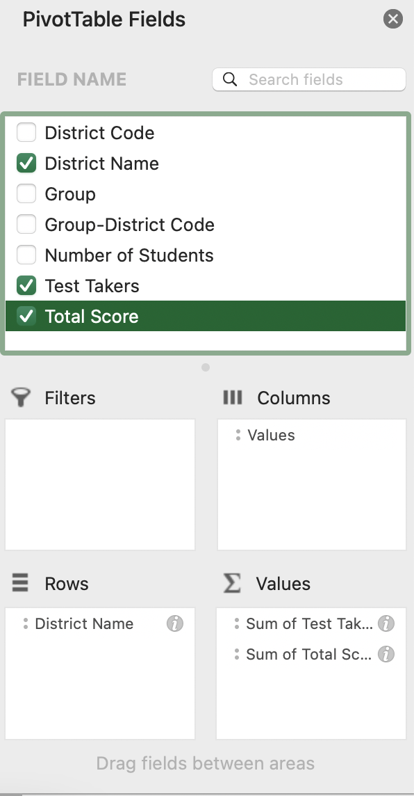
Step 4
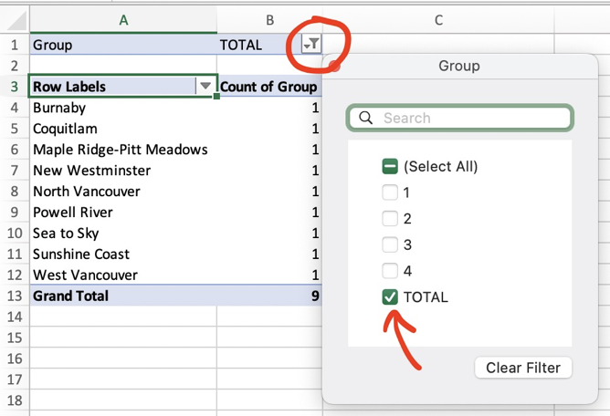
- Select
Groupfield name and move it to the Filter area. In the filter above, unselect the “TOTAL” option. - Where to find a filter:
Step 5
In the Values area, change the Total Score from Sum to the Average.
Hint: Click on the info symbol to change the aggregation function:

Visualizations
How to make a simple visualization
Step 1
Return to the Data sheet
Step 2
Select only TOTAL rows using filters for Group
Step 3
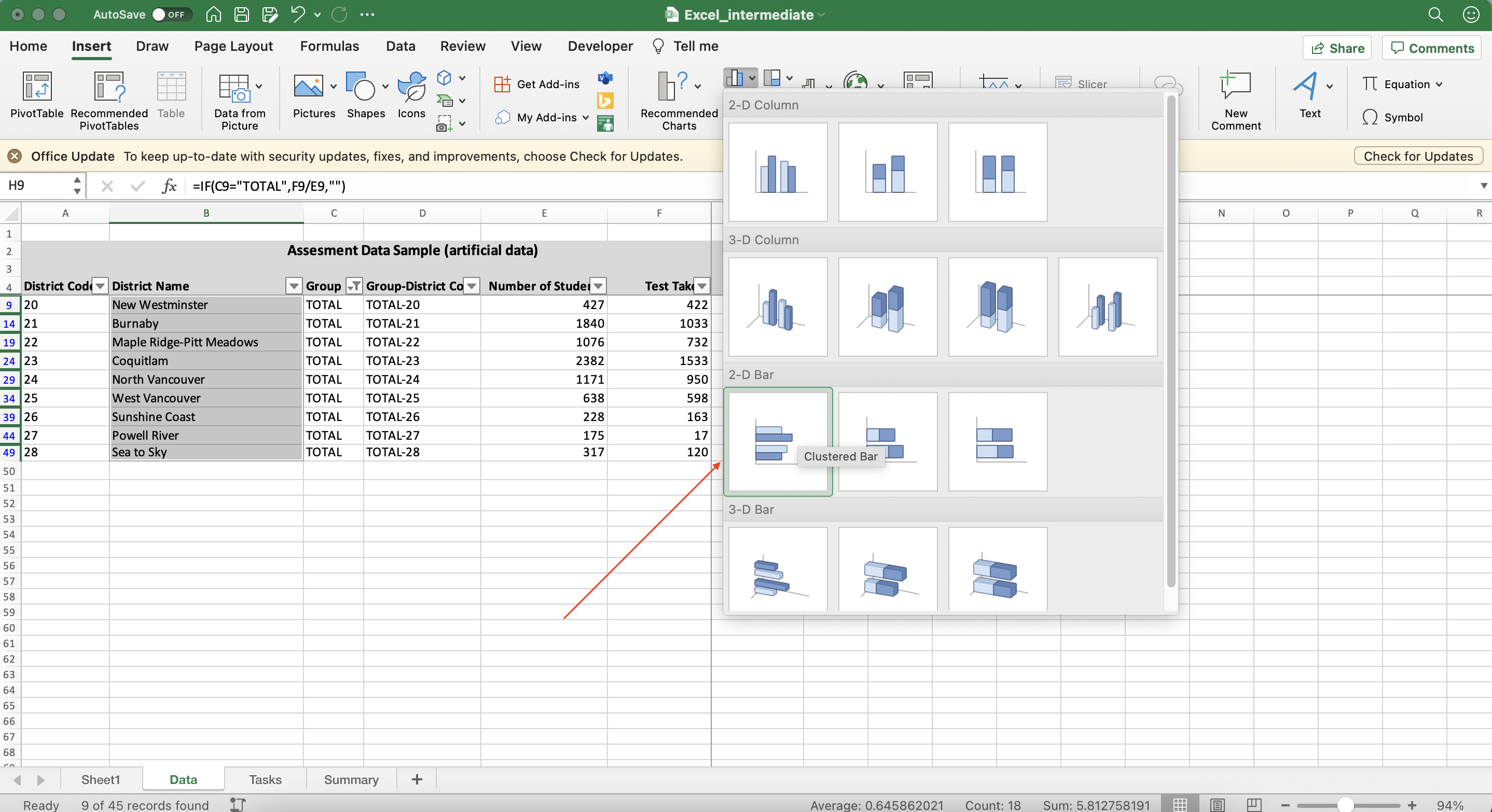
Select columns District Name and Percent of Test Takers.
Hint: Hold CTRL or CMD to select both columns;
Step 4
In the Insert menu select 2D horizontal bar chart (Clustered Bar).
Advice: Horizontal bar chart is a preferred when having categories with long names
Step 5
Sort bins by sorting the Percent of Test Takers column.
Advice: Sorting/filtering the original data has a direct impact on the visualization.
Link: How-tos on plotting different graph types in Excel
Data Series in Visualizatons
Adding average line
Step 1
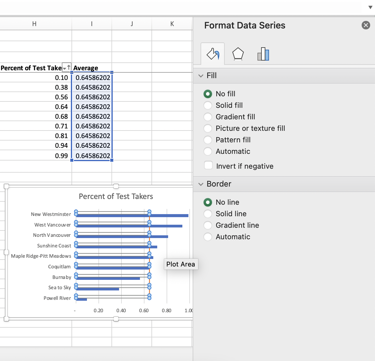
Create new column named Average. Use previously learned SUBTOTAL to get the average Percent of Test Takers and fill the whole column with this value
Answer (click to open)
`SUBTOTAL(1,H$9:H$49)`
Step 2
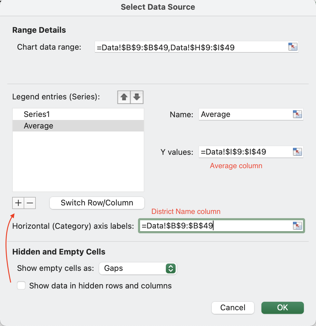
Right click on the existing visualization, choose Select Data and add another series (in the Legend Series click on the plus button);
Step 3
Select Average as Y-values, Average column name as Name, and District Name column as X-values. You should have another set of bins added to your visualization;
Step 4
Select series corresponding to average (click on the orange bins). You can Change Series Chart Type by clicking right button and selecting Combo. However, this option only supports vertical bar chart.
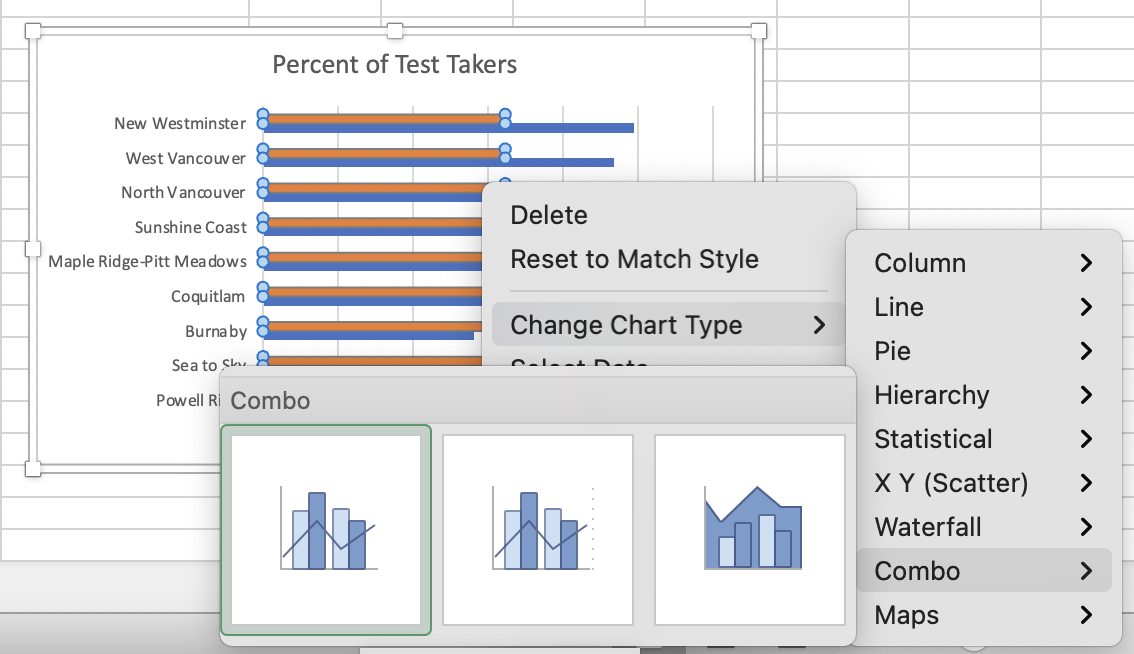
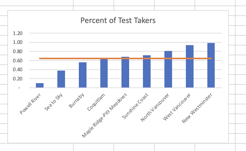
There are some workarounds available. For example, you can add linear trend line (select series, go to Chart Design) and click Add Chart Element -> Trend Line -> Linear (or right click and select Add Trendline)
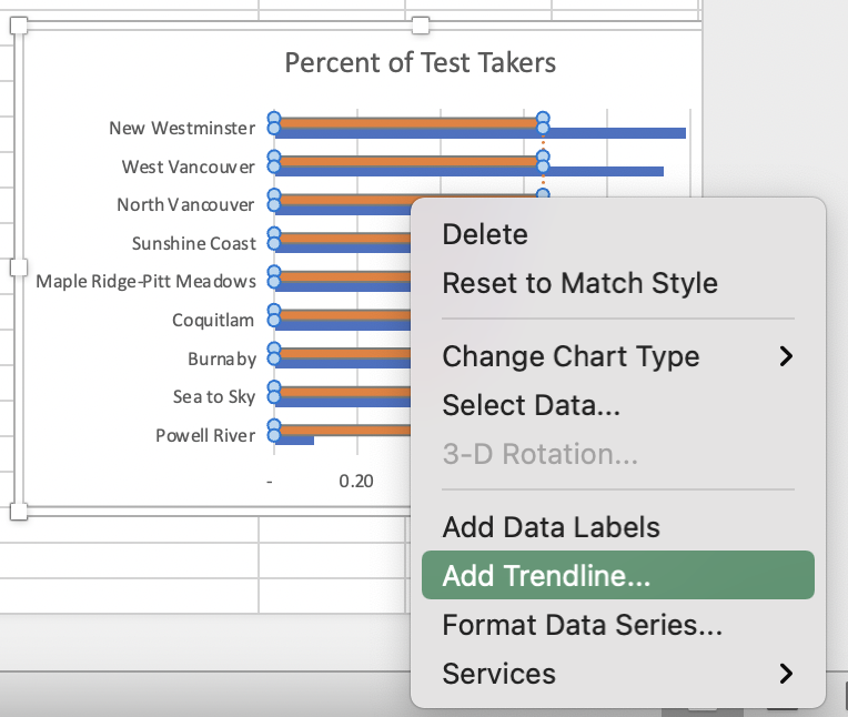
It will create vertical line for the average, just like we wanted. Now, you can make your bins invisible. Either in the Format menu or Format pane, select Fill -> No Fill and Border (or Shape Outline) -> No line.
Saving your chart
Save Visualization
Step 1
Select Chart Area (be careful not to select the Plot Area instead), right click and select Save as Picture to save your visualization