Census Data
Nothing stops us from adding more data to our variables. In this section, we will make use of data from the 2016 census containing the information about income for certain salary ranges.
The 2016 Census data is quite verbose, so I took the liberty to pre-process and normalize the data in the two variables below, income_100k and income_30k. These variables represent the ratio of people in a certain neighborhood from a certain age group who reported having salaries above 100K or below 30K, respectively.
R Code
income_100k <- c(
  0.18, 0.19, 0.15, 0.09, 0.08, 0.09, 0.15,
  0.25, 0.11, 0.10, 0.24, 0.21, 0.08, 0.18,
  0.18, 0.06, 0.08, 0.13, 0.15, 0.05, 0.06,
  0.23)

income_30k <- c(0.15, 0.11, 0.11, 0.18, 0.23,
  0.20, 0.15, 0.11, 0.27, 0.17, 0.11, 0.14,
  0.20, 0.12, 0.14, 0.25, 0.21, 0.13, 0.16,
  0.25, 0.25, 0.11)
Adding Census Data to our Variable
When we write vancouver_boundaries$ ... you can replace the ... by a field available in your dataset to check its values.
You can also create a new field if it doesn’t exist:
R Code
vancouver_boundaries$income_100k <- income_100k * 100
vancouver_boundaries$income_30k <- income_30k * 100
1 Dividing Data into Buckets
We want to divide the income into buckets so it is easier to identify different populations. We can do that with the classIntervals function
R Code
brks <- classIntervals(vancouver_boundaries$income_100k, n = 5, style = "quantile")
brks
Output
> brks
style: quantile
  one of 715 possible partitions of this variable into 5 classes
    [5,8)  [8,10.4) [10.4,15) [15,18.8) [18.8,25]
        3         6         2         6         5
2 Plotting Income Data
Now that we have intervals and numerical data, i.e., income_100k, we can use that in our plot to quickly identify regions in each bucket.
R Code
tm_shape(vancouver_boundaries) +
  tm_polygons("income_100k",
              palette = "RdYlGn",  breaks= brks$brks,
              title="Income (%)", border.col = "white") +
  tm_text("mapid", just = "center", size = 0.8) +
  tm_legend(outside=TRUE)
Output
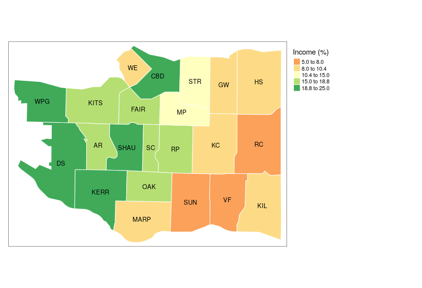
Choropleth maps
Choropleth maps (choro = area and pleth = value) aggregates some attribute (e.g., income) over a defined area (e.g., neighborhoods)
Is anything Wrong with this Map?

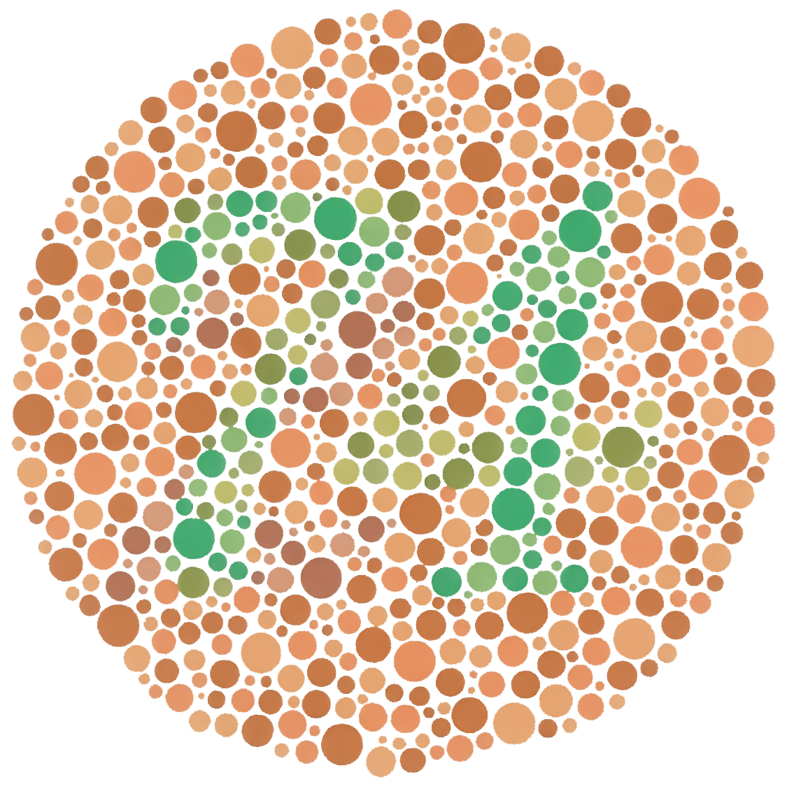
3 Consider colour-blind or printer-friendly palettes
R Code
display.brewer.all(n = NULL, type = "all", select = NULL, colorblindFriendly = TRUE)
4 We can change the palette of our map accordingly
R Code
tm_shape(vancouver_boundaries) +
  tm_polygons("income_100k",
              palette = "GnBu",  breaks= brks$brks,
              title="Income (%)", border.col = "white") +
  tm_text("mapid", just = "center", size = 0.8) +
  tm_legend(outside=TRUE)
Recap
1 classIntervals divides the data into intervals
2 tm_polygons can use numerical data as one of its parameters, the breaks parameter divides the data according to the intervals we have defined
3 display.brewer.all displays different colours palettes
4 palette sets a specific palette to our plot