Spatial correlation

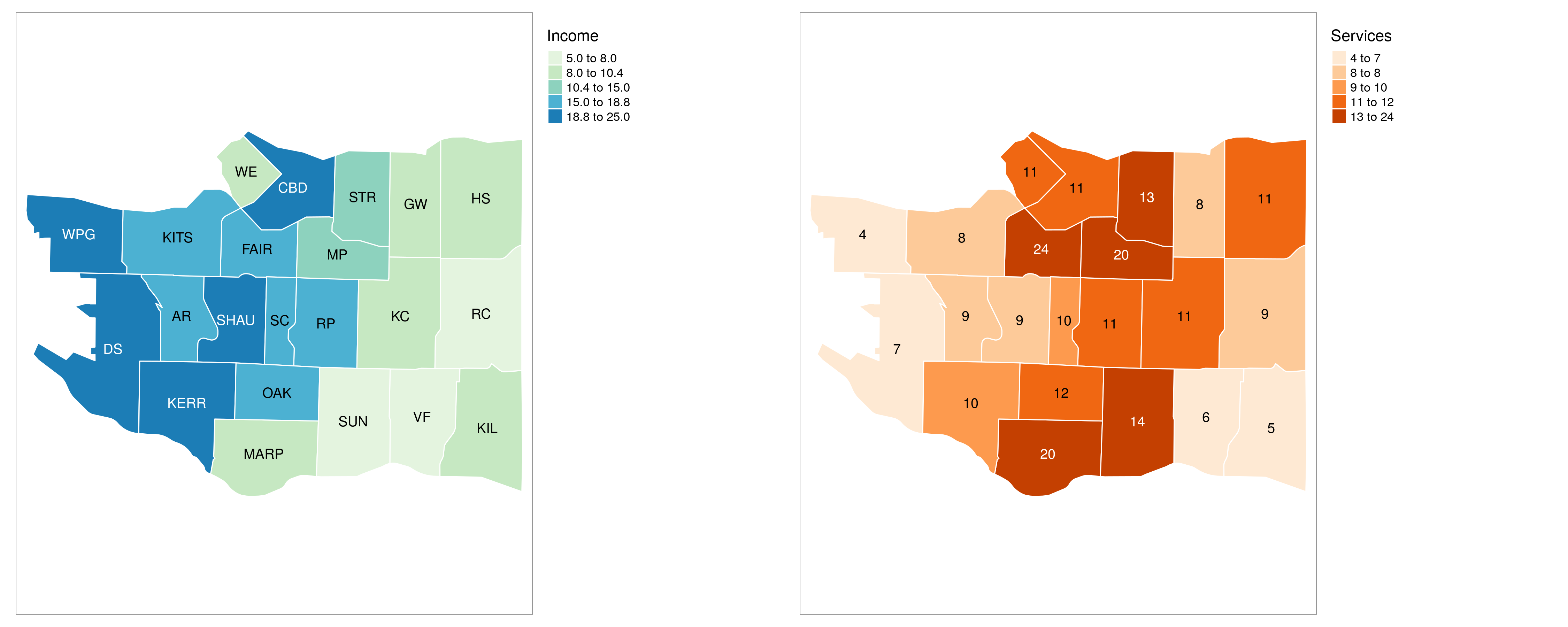
Income for every Neighbourhood

Let’s review the income for every region

R Code

brks <- classIntervals(vancouver_boundaries$income_100k, n = 5, style = "quantile")
plt1 <- tm_shape(vancouver_boundaries) + 
  tm_polygons("income_100k", border.col = "white", palette = "GnBu", breaks= brks$brks, title="Income") +
  tm_text("mapid", just = "center", size = 0.8) +
  tm_legend(outside=TRUE)
plt1

Services for every Neighbourhood

Let’s count the number of points in every neighbourhood

We explain counting services at dplyr

R Code

cnt_services <- function(point_data) {
  lst_cnt <- c()
  for (neighbourhood in vancouver_boundaries$mapid) {
    neighbourhood_polygon <- vancouver_boundaries %>% filter(mapid == neighbourhood)
    cnt <- lengths(st_intersects(neighbourhood_polygon, point_data))
    lst_cnt <- c(cnt, lst_cnt)
  } 
  
  return(lst_cnt)
}

vancouver_boundaries$schools <- cnt_services(schools)
vancouver_boundaries$libraries <- cnt_services(libraries)
vancouver_boundaries$community_centres <- cnt_services(community_centres)

vancouver_boundaries$all_services <- vancouver_boundaries$schools + 
  vancouver_boundaries$libraries + 
  vancouver_boundaries$community_centres

R Code

brks <- classIntervals(vancouver_boundaries$all_services, n = 5, style = "quantile")
plt2 <- tm_shape(vancouver_boundaries) + 
  tm_polygons("all_services", border.col = "white", palette = "Oranges", breaks= brks$brks, title="Services") +
  tm_text("all_services", just = "center", size = 0.8) +
  tm_legend(outside=TRUE)
plt2

Images side by side

We can plot images side-by-side with tmap_arrange

R Code

current.mode <- tmap_mode("plot")
tmap_arrange(plt1, plt2)
tmap_mode(current.mode)

Output

1 Is there any correlation between income and services in a neighborhood

It’s time to check whether there is any correlation between income in a neighbourhood and its services. We can use the cor.test for that.

R Code

cor.test(vancouver_boundaries$income_30k, vancouver_boundaries$all_services, method="pearson")

Output

> cor.test(vancouver_boundaries$income_100k, vancouver_boundaries$all_services, method="pearson")

	Pearson's product-moment correlation

data:  vancouver_boundaries$income_100k and vancouver_boundaries$all_services
t = -0.82768, df = 20, p-value = 0.4176
alternative hypothesis: true correlation is not equal to 0
95 percent confidence interval:
 -0.5605809  0.2595383
sample estimates:
       cor 
-0.1819834 

Given the p-val above, we cannot assume that there are more or less services in a region given its income.

source

Recap

1 cor.test is used to evaluate the association between two or more variables.