Thematic Mapping QGIS
As a reminder, thematic maps visualize specific aspects of a dataset across space. Or, as Statistics Canada puts it: “A thematic map shows the spatial distribution of one or more specific data themes for standard geographic areas.” As reviewed yesterday, there are different kinds of thematic maps each suiting a different purpose.
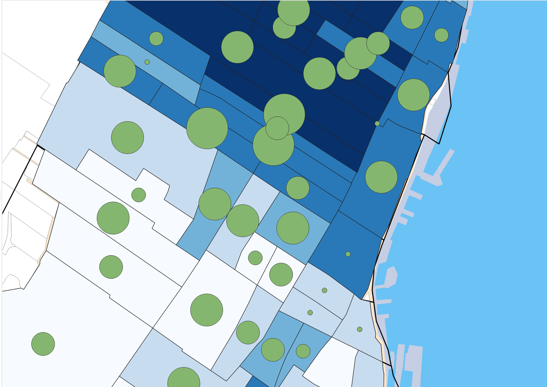
This afternoon, you will learn how to make 2 of the most commonly used thematic visualizations: a choropleth map and a proportional symbol map. While this morning you practiced downloading your own data and creating a QGIS project from scratch, for thematic mapping, we’ve prepared a project for you. We will be using historic data for Montréal to visualize the spatial distribution and density of French Canadians according to the 1881 census.
Today’s data
To Do
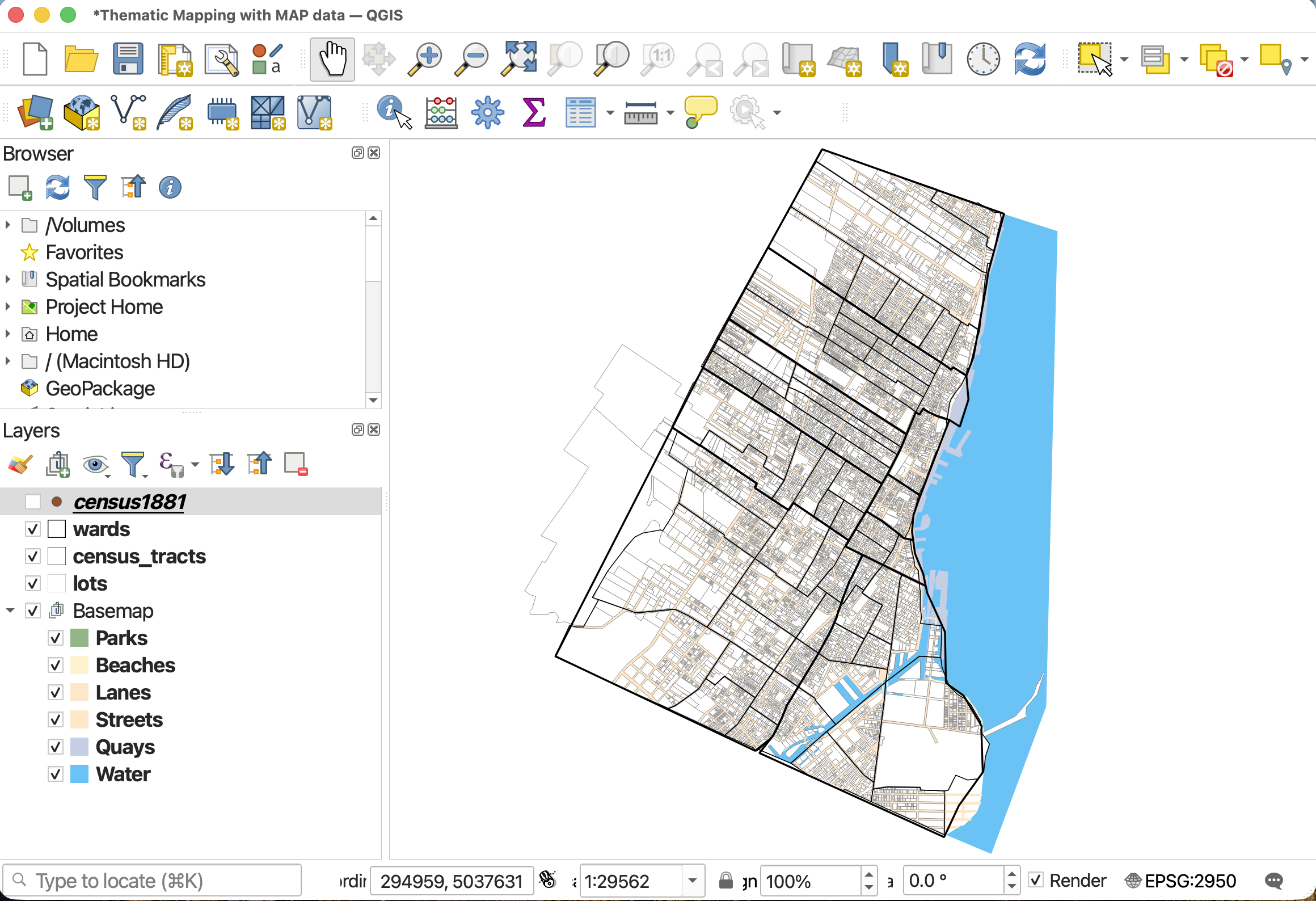
Launch the thematic-mapping.qgz project in the folder dhsi-workshop/Day2/thematic-mapping. You will see the following layers loaded.
The data for today’s lesson is from the public history project Montréal, l’avenir du passé (MAP), directed by Sherry Olson and Robert C.H. Sweeny. Translating to Montréal, The Future of the Past, MAP digitizes, geocodes, and georeferences data from historical atlases, city directories, census records, and municipal tax rolls to show demographic change over time and space in Montréal. For more about the MAP project
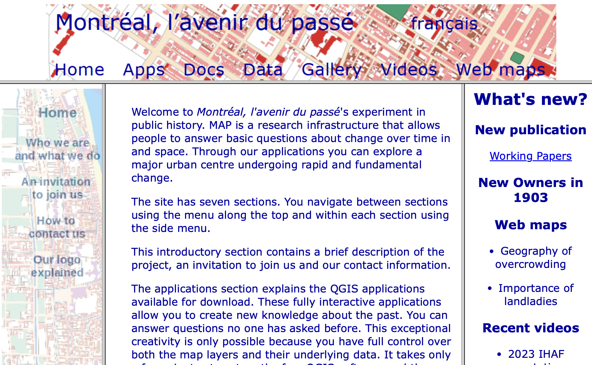
As a public history project, MAP makes their spatial datasets freely available and their entire website and documentation is bilingual (French & English). Not only that, they have prepared QGIS applications which visualize selected data. You can simply download one of these “apps” and explore a given time period. MAP is therefore an exceptional example of digital humanities using GIS! And QGIS, for that matter!!
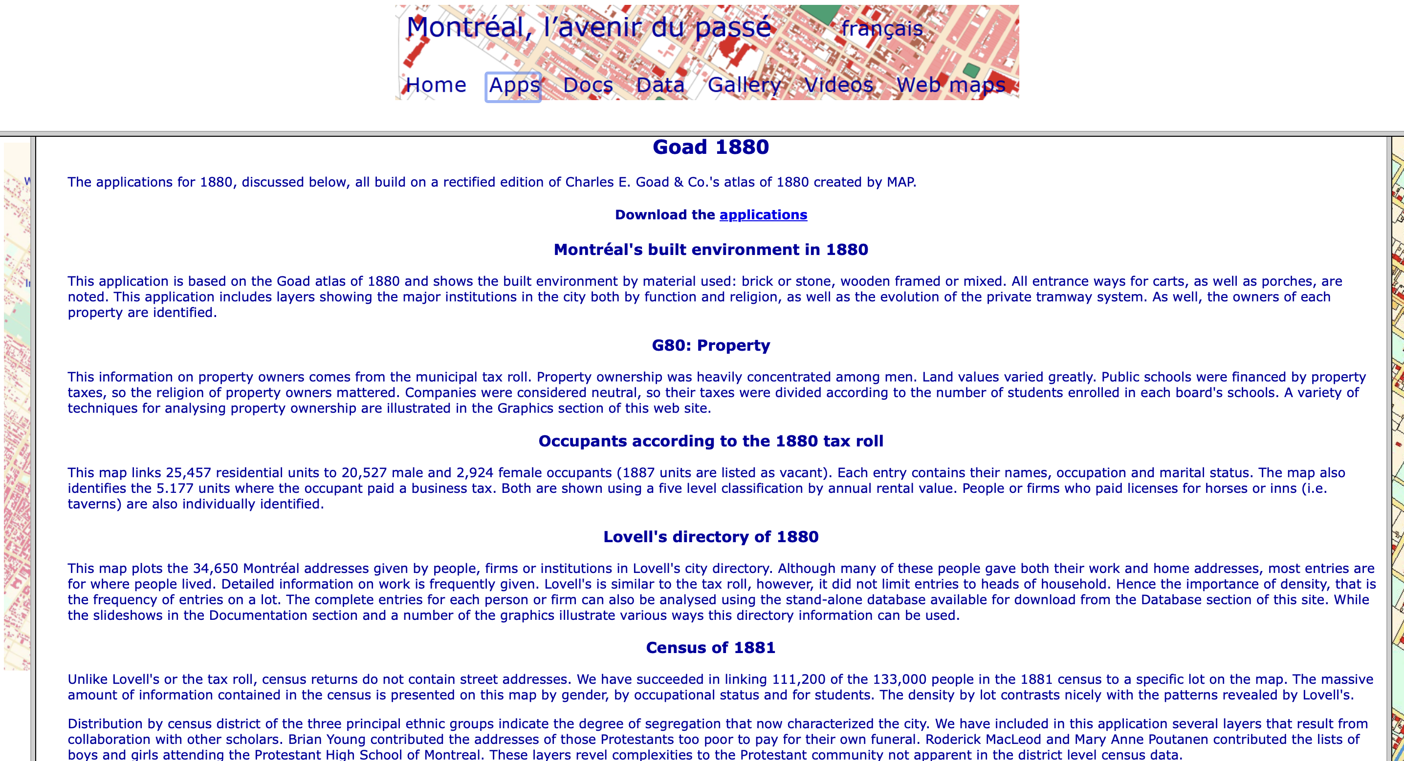
MAP has enthusiastically encouraged us to use their data in this DHSI workshop, but we highly recommend exploring their datasets and prepared QGIS applications directly. Today’s exercises will work with data available in the Goad 1880 applications which “build on a rectified edition of Charles E. Goad & Co.’s atlas of 1880 created by MAP.” This download contains multiple QGIS projects and data all from 1880-1881. While physical features such as water, streets, and buildings come from the 1880 Goad Atlas, administrative data on lots, wards, and census tracts — and of course census data itself — come from the 1881 Census. Data on occupants and business rents comes from the 1880 Municipal tax roll, and further demographic information comes from Lovell’s directory of 1880-81.
More about the MAP project can be found on the Centre interuniversitaire d’études québécoises (CIEQ) website: https://map.cieq.ca/. This site is tailored less towards downloading and playing with datasets than exploring them online. For instance, mix and match variables, how people made a living, street crawling, or just look at Lovell Directory data in web map form! For more on their sources, see the CIEQ website subpages “Our Gorgeous Sources” and “In the Storeroom”.
What we’ll use…
Below we’ve outlined the data used in today’s lesson with a description of what it visualizes as well as, for reference, what it’s named in the Goad 1880 MAP application download and any modifications made to the original dataset. Data was renamed for ease of understanding.
All the data we’ll use is stored in shapefile format. While QGIS projects within the Goad 1880 MAP application download were set to the projection NAD83(CSRS) / MTM zone 8, individual shapefiles were not stored with projections but rather “projected on the fly” when loaded into a project. Therefore, all renamed shapefiles were also saved with the Coordinate Reference System (CRS) NAD83(CSRS) / MTM zone 8. The only difference this makes is in the kinds of sidecar files associated to a shapefile.
Demographic data
census1881Demographic data from the 1881 Census containing 111,208 features, with information on name, age, sex, occupation, religion, disability (‘blind’, ‘deaf’, ‘dumb’, ‘unsound’), birth place, and more. The geographical tie is at the lot level, and while the full census contained some twenty thousand more responses, MAP was only able to successfully link 111,208 at the lot level (quite impressive!). This data layer is namedg80cen81in MAP’s Goad 1880 application download.
Administrative Boundaries/Units
-
lotsIndividual lots according to the 1881 Census. Containing 12,226 features, this layer was originally namedcensusltin MAP’s Goad 1881 applications download.censusltis geographically nearly identical tonewlots81, the latter containing one more feature. However, the two datasets differ in attribute tables.censusltwas chosen for our exercises because it has a fewer attributes and thus a cleaner attribute table. Bothcensusltandnewlots81differ from the dataset for lots used in MAP QGIS applications which visualizeg80_lots. This dataset has a few hundred fewer lots, and differences are especially apparent around the waterfront. Because we will be visualizing census data, lots for our workshop are based on census lots. -
wardsWards from the 1881 Census. This data layer is also namedwardsin MAP’s Goad 1880 applications download. -
census_tractsCensus tracts 1881 Census. This data layer is namedctractsin MAP’s Goad 1880 applications download. To see visualizations specific to this administrative/census level see the QGIS ProjectCensus returns 1881.qgsin MAP’s Goad 1880 applications download.
Contextual Features
Physical and infrastructural features are organized into the data subfolder features. These layers are parks, beaches, lanes, streets, quays, and water. Each shapefile was slightly renamed for consistency and saved them with a projection. Additionally, the water dataset was modified to rectify an issue with the geometry in the canal feature.
You’ll notice when you open the QGIS project for today that the files for contextual features are already loaded — if hidden — in the project. This is because MAP went to great efforts to curate a symbology for this basemap data that works well, and re-loading them to our project would require we do all this work over again. This way, we can simply turn on the layer group when we are ready to map.
Alright! Now that we understand what data we’re using and where it came from, Let’s move on to practicing thematic mapping with QGIS!
Resources for Thematic Mapping
- Axis Map’s Guide
- ColorBrewer is a fantastic resource for generating customized color palettes.
- Coloring for Colorblindness for colorblind-friendly palettes.
- Axis Map’s guide to Choropleth Maps
- Axis Map’s guide to Proportional Symbols
- Axis Map’s guide to Dot Density Maps
- Axis Map’s guide to Cartograms
- Axis Map’s guide to Univariate vs Multivariate Maps
- Perceptual Scaling of Map Symbols by John Krygier.
- Another UBC Research Common’s tutorial on Proportional Symbol Mapping, including guide to sizing proportional symbols by hand in an illustration software.
- Axis Map’s guide to Data Classification
- UBC Research Commons tutorial on making Heatmaps with QGIS
- UBC Research Commons tutorial on making Cartograms with QGIS
Table of contents
Loading last updated date...